1. Preparing State, County, Fips, and Center Data
ggplot2 package is known for its beautiful plots in R, such as histograms, boxplots, scatter plots etc. However, one can do geospatial mapping as well with this package. Here we’ll first build the data step by step using map_data and fips data, and then use the geom_polygon that will enable us to perform geospatial mapping.
The ggplot2::map_data function has the polygon data of longitudes, and latitudes imported from the maps package.
State and County Polygon Data
# Import libraries
library(tidyverse)
library(data.table)
library(DT)
library(knitr)
library(stringr)
Let’s first check whether there are some counties which have special endings such as: city, county, parish.
x = map_data('county') %>% as.data.table()
setnames(x, c('region', 'subregion'), c('state','county'))

d_city = x[county %>% str_detect('city'), .(group = unique(group)), keyby = .(state, county)]
d_city
## state county group
## 1: maryland baltimore city 1183
## 2: missouri st louis city 1545
## 3: nevada carson city 1731
## 4: virginia charles city 2809
## 5: virginia james city 2837x[county %>% str_detect('county'), .N]## [1] 0x[county %>% str_detect('parish'), .N]## [1] 0v_without_city = str_replace(d_city$county, 'city', '') %>%
str_trim(side = 'right')
d_city[, without_city := v_without_city]
v = list()
for (i in seq(nrow(d_city)) ) {
counties = x[state == d_city[i = i, state], unique(county)]
present = str_detect(string = counties, pattern = d_city$without_city[i])
v[[i]] = data.table(state = d_city$state[i], county = counties[present])
}
rbindlist(v) %>% datatable()fun_load_polygon = function(map_type) {
x = map_data(map = map_type) %>% as.data.table()
setnames(x, c('region', 'subregion'), c('state', 'county'))
x2 = x[, .(state, county)] %>%
map_df(.f = str_to_lower) %>%
map_df(.f = str_replace_all, pattern = '[[:punct:]]', replacement = '') %>%
map_df(.f = str_replace_all, pattern = '[[:space:]]', replacement = '') %>%
as.data.table()
if (map_type == 'county') {
x2[state == 'districtofcolumbia' & county == 'washington',
county := 'districtofcolumbia']
x2[state == 'montana' & county == 'yellowstonenational',
county := 'yellowstone']
}
x$state = x2$state
x$county = x2$county
return(x)
}
polygon_state = fun_load_polygon('state')
polygon_county = fun_load_polygon('county')
polygon_state[1:1000, ] %>% datatable(caption = 'State Polygon', rownames = F)polygon_county[1:1000, ] %>% datatable(caption = 'County Polygon', rownames =F)# polygon_county[state == 'montana' & county == 'yellowstone']
# polygon_county[state == 'montana' & county == 'park']The punctutations and spacings have been removed, and the names have been converted to all lower case. The aim of this is to make the datasets as universal as possible, so that they can be merged with other datasets easily.
One interesting fact that I found out is that county Chesapeake in Virginia is not present in the county polygon data, but is present in state polygon data. However, Chesapeake in state polygon data is named wrong, and here together with Chincoteague represents the northern peninsula of Virginia that stretches to Maryland. It is actually the counties of Accomack, and Northampton. This peninsula is shown in the map below. So, it should not be confused with the real Chesapeake.
ggplot(data = polygon_state[state == 'virginia'], mapping = aes(x = long, y = lat, group = group)) +
    geom_polygon(fill = 'ivory1', color = "limegreen", size = 0.1) +
    geom_polygon(data = polygon_state[county %in% c('chesapeake', 'chincoteague')], col = 'black', size = 2) +
    geom_polygon(data = polygon_county[state == 'virginia' & county %in% c('accomack', 'northampton')], aes(fill = county)) +
    coord_map('mercator') +
    theme_bw()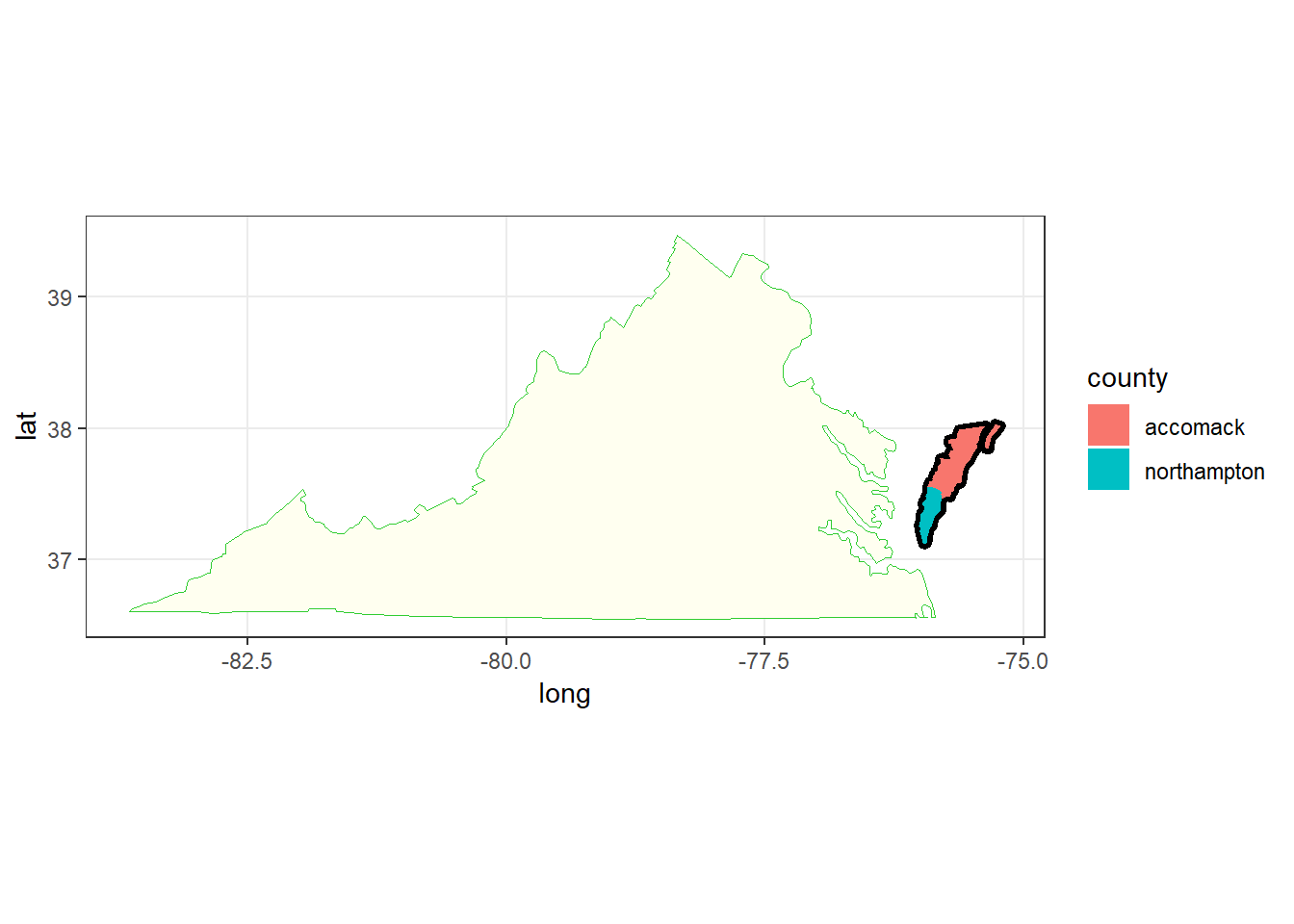
The county name “Washington” within the state of “District of Columbia” has been renamed to “District of Columbia”, and the county name “Yellowstone National” has been renamed to “Yellowstone”, as these names are more common in databases. Depending on your data that contains the values to be analyzed, one can play with the names of the counties to match them. Even better, using a common unique identifier can help in the process and decrease the chances of making an error. Fips is such a unique identifier used in the geographical mapping of state and county data. States and counties each have their own unique fips code.
Next step will involve the process of preparing the fips data. Maps package in R contains the county fips dataset.
Fips Data
library(maps)
data("county.fips")
head(county.fips) %>% kable()| fips | polyname |
|---|---|
| 1001 | alabama,autauga |
| 1003 | alabama,baldwin |
| 1005 | alabama,barbour |
| 1007 | alabama,bibb |
| 1009 | alabama,blount |
| 1011 | alabama,bullock |
county.fips = str_split(string = county.fips$polyname, pattern = ',', simplify = T) %>%
    as.data.frame() %>%
    map_df(.f = str_to_lower) %>%
    map_df(.f = str_replace_all, pattern = '[[:punct:]]', replacement = '') %>%
    map_df(.f = str_replace_all, pattern = '[[:space:]]', replacement = '') %>%
    cbind(county.fips$fips) %>%
    as.data.table() %>%
    setnames(c('state', 'county', 'fips'))

county.fips %>% datatable()Let’s check whether the fips data has some common suffixes at the end of counties:
# Suspecting for some counties having suffixes such as:
x = county.fips
d_city = x[county %>% str_detect('city'), .SD]
d_city
## state county fips
## 1: maryland baltimorecity 24510
## 2: missouri stlouiscity 29510
## 3: nevada carsoncity 32510
## 4: virginia charlescity 51036
## 5: virginia jamescity 51095d_county = x[county %>% str_detect('county'), .SD]
d_county## Empty data.table (0 rows) of 3 cols: state,county,fipsd_parish = x[county %>% str_detect('parish'), .SD]
d_parish## Empty data.table (0 rows) of 3 cols: state,county,fipsd_main = x[county %>% str_detect('main'), .SD]
d_main## state county fips
## 1: florida okaloosamain 12091
## 2: northcarolina currituckmain 37053
## 3: texas galvestonmain 48167
## 4: virginia accomackmain 51001
## 5: washington piercemain 53053fun_counties_with_extra_names = function(d = county.fips, d_extra, extra = 'main') {
v_without = str_sub(d_extra$county, 1, str_length(d_extra$county) - str_length(extra))
counties_extra = list_along(v_without)
for (i in seq_along(v_without)) {
counties_extra[[i]] = d[county %>% str_detect(v_without[i]) &
state == d_extra[i, state], .SD]
}
return(data.table::rbindlist(counties_extra))
}Counties in the fips set do not end with either county or parish.
Counties that have city as their ending:
extra = 'city'
county_extra = fun_counties_with_extra_names(d = county.fips,
                                             d_extra = d_city, extra)
county_extra %>% datatable()Counties that have main as their ending:
extra = 'main'
county_extra = fun_counties_with_extra_names(d = county.fips,
                                             d_extra = d_main, extra)
county_extra %>% datatable()Let’s first get rid of the extra entries for counties with main.
fun_clean_counties_with_extra_names = function(d, d_extra, extra = 'main') {
    # get rid of any county that has "extra" and other suffixes
    d = d[!fips %in% county_extra$fips]
    # get rid of "extra" part of counties
    d_extra$county = str_sub(d_extra$county, 1, str_length(d_extra$county) - str_length(extra))
    # append it to county.fips data
    return( rbind(d, d_extra) )
}

extra = 'main'
county.fips = fun_clean_counties_with_extra_names(d = county.fips,
                                                  d_extra = d_main, extra)
Now, let’s check whether there are any other duplicates.
dup = county.fips[duplicated(x = county.fips$fips), fips ]
county.fips[fips %in% dup, ]
## state county fips
## 1: louisiana stmartinnorth 22099
## 2: louisiana stmartinsouth 22099
## 3: montana park 30067
## 4: montana yellowstonenational 30067
## 5: washington sanjuanlopezisland 53055
## 6: washington sanjuanorcasisland 53055
## 7: washington sanjuansanjuanisland 53055county.fips[county %in% c('yellowstone', 'park') & state == 'montana', ] %>% kable()| state | county | fips |
|---|---|---|
| montana | park | 30067 |
| montana | yellowstone | 30111 |
Indeed there are other duplicate entries. Let’s clean these remaining duplicates. It is found out Yellowstone in Montana has fips code 30111. From other datasets it is also verified that county Park in Montana has fips code 30067. Thus, for the repeated values in Montana, the one to be kept is Park.
county.fips[fips == 22099, county := 'stmartin']
county.fips[fips == 30067, county := 'park']
county.fips[fips == 53055, county := 'sanjuan']
county.fips = county.fips[!duplicated(county.fips)]

county.fips[duplicated(county.fips$fips)]
## Empty data.table (0 rows) of 3 cols: state,county,fipscounty.fips[state == 'districtofcolumbia', county := 'districtofcolumbia']Finally the fips dataset is clean and ready to be integrated into the polygon data.
Now, I will join the county polygon data with the fips code and save for later use. Since the polygon_county data’s counties match one to one with the ones at county.fips, we can join these to reach the desired dataset.
polygon_county[, .(county = unique(county)), by = state][, county] %>%
    setdiff( county.fips[, county])
## character(0)polygon_county = left_join(polygon_county, county.fips,
by = c('state', 'county')) %>% as.data.table()
polygon_county[is.na(fips)]## Empty data.table (0 rows) of 7 cols: long,lat,group,order,state,county...polygon_county[1:1000] %>% datatable()Good. We have cleaned the fips data and joined with the cleaned polygon data.
Center Data
The final step involves computing the center latitude and longitude of states and counties. This sort of data can be useful when we want to plot something in the center of states or counties.
# Input data is the polygon data
# d has long and lat variables for the state-county combinations (or fips)
fun_get_centers = function(d) {

    # d[, .(atan2( sum(cos(long)), sum(cos(lat)) ) )]
    d = copy(d)
    d[, `:=`(long_rad = long*pi/180, lat_rad = lat*pi/180)]

    xyz = d[, .( x = mean( cos(lat_rad) * cos(long_rad) ),
                 y = mean( cos(lat_rad) * sin(long_rad) ),
                 z = mean( sin(lat_rad) ) ), by = .(state, county, group)]

    # central_long = atan2(y,x)
    # central_square_root = sqrt(x^2 + y^2)
    # central_lat = atan2(z, central_square_root)

    xyz = xyz[, {
                    cent_long = atan2(y,x)
                    cent_sqrt = sqrt(x^2 + y^2)
                    cent_lat  = atan2(z, cent_sqrt)

                    cent_lat = cent_lat * 180/pi
                    cent_long = cent_long * 180/pi

                    list(long = cent_long,
                         lat = cent_lat)


              }, by = .(state, county, group)]

    return(xyz)

}

center_county = fun_get_centers(polygon_county)
center_state = fun_get_centers(polygon_state)

center_county = left_join(center_county, county.fips) %>% as.data.table()
dup = center_county[duplicated(center_county$fips), fips]
center_county[fips %in% dup,] %>% kable()| state | county | group | long | lat | fips |
|---|---|---|---|---|---|
| florida | okaloosa | 335 | -86.56789 | 30.58918 | 12091 |
| florida | okaloosa | 336 | -86.45881 | 30.43240 | 12091 |
| louisiana | stmartin | 1128 | -91.72565 | 30.23448 | 22099 |
| louisiana | stmartin | 1129 | -91.28414 | 29.84270 | 22099 |
| montana | yellowstone | 1620 | -108.18860 | 46.02341 | 30111 |
| montana | yellowstone | 1621 | -110.75128 | 44.98961 | 30111 |
| northcarolina | currituck | 1883 | -75.95462 | 36.52606 | 37053 |
| northcarolina | currituck | 1884 | -75.96341 | 36.35219 | 37053 |
| northcarolina | currituck | 1885 | -75.70764 | 36.11839 | 37053 |
| texas | galveston | 2575 | -95.04942 | 29.46282 | 48167 |
| texas | galveston | 2576 | -94.56639 | 29.52865 | 48167 |
| virginia | accomack | 2790 | -75.31457 | 37.94509 | 51001 |
| virginia | accomack | 2791 | -75.69053 | 37.72515 | 51001 |
| washington | pierce | 2917 | -122.05552 | 47.02515 | 53053 |
| washington | pierce | 2918 | -122.66869 | 47.31016 | 53053 |
| washington | sanjuan | 2919 | -122.82764 | 48.45774 | 53055 |
| washington | sanjuan | 2920 | -122.83491 | 48.64715 | 53055 |
| washington | sanjuan | 2921 | -123.02817 | 48.52786 | 53055 |
center_county[is.na(fips)]## Empty data.table (0 rows) of 6 cols: state,county,group,long,lat,fips# fwrite(polygon_county, str_c(files_dir, 'polygon_county.csv'))
# fwrite(polygon_state, str_c(files_dir, 'polygon_state.csv'))
# fwrite(center_county, str_c(files_dir, 'center_county.csv'))
# fwrite(center_state, str_c(files_dir, 'center_state.csv'))It should be noted that 8 counties are divided by waterways, and thus have different groupings of polygon values. They are not duplicate records. This can also be seen in the center_state data. There is also no missing fips code in the polygon set. So the center_county and center_state datasets are clean and ready for analysis.